Discrete (arbitrary gradient moment) EPG in 3D#

In the 3D discrete EPG model (C++, Python), the gradient moments may vary across time intervals as in regular EPG, but their amplitude is specified on the three spatial axes. The class interface is similar to the two other models.

The following code sample simulates a idealized PGSE diffusion sequence in an anisotropic medium and shows the dependency of the signal attenuation to the relative orientation of diffusion tensor and of the diffusion gradient.

Python

import numpy
import sycomore
from sycomore.units import *
import vtk
import vtk.numpy_interface.dataset_adapter

species = sycomore.Species(
    1000*ms, 100*ms, numpy.diag([2000, 500, 100])*um**2/s)

TE = 50*ms
b = 2000*s/mm**2

# Assuming Δ = δ (i.e. we can neglect the duration of the RF pulse, the spatial
# encoding gradients and the crusher gradients, and the diffusion gradient is
# on all the time, we get b = (γGδ)² ⋅ (2δ/3) with δ=TE/2.
G = (b/(sycomore.gamma**2 * 2/3 * (TE/2)**3))**0.5
print(f"G={numpy.round(G.convert_to(mT/m)):.0f} mT/m")

def dw_se(species, TE, G):
    model = sycomore.epg.Discrete3D(species)
    
    # Excitation
    model.apply_pulse(90*deg)
    
    # Diffusion-sensitization gradient is on all the time before the refocussing
    model.apply_time_interval(TE/2, G)
    
    # Refocussing
    model.apply_pulse(180*deg)
    
    # Diffusion-sensitization gradient is on all the time before TE
    model.apply_time_interval(TE/2, G)
    
    return numpy.abs(model.echo)

# Generate a unit sphere
sphere_source = vtk.vtkSphereSource()
sphere_source.SetRadius(1)
sphere_source.SetThetaResolution(50)
sphere_source.SetPhiResolution(50)
sphere_source.Update()
sphere = vtk.numpy_interface.dataset_adapter.WrapDataObject(
    sphere_source.GetOutput())
print(len(sphere.Points), "points on sphere")

# Simulate the sequence with a diffusion gradient along each point on the sphere
S_0 = dw_se(species, TE, [0*mT/m, 0*mT/m, 0*mT/m])
attenuation = numpy.zeros((len(sphere.Points))) 
for index, direction in enumerate(sphere.Points):
    S = dw_se(species, TE, direction*G)
    attenuation[index] = S/S_0
    sphere.Points[index] *= attenuation[index]

C++

#include <iostream>

#include <sycomore/epg/Discrete3D.h>
#include <sycomore/Species.h>
#include <sycomore/sycomore.h>
#include <sycomore/units.h>

#include <xtensor/xbuilder.hpp>

using namespace sycomore::units;

sycomore::Real dw_se(
    sycomore::Species const & species, sycomore::Quantity const & TE,
    sycomore::Vector3Q const & G)
{
    sycomore::epg::Discrete3D model(species);
    
    // Excitation
    model.apply_pulse(90*deg);
    
    // Diffusion-sensitization gradient is on all the time before the refocussing
    model.apply_time_interval(TE/2, G);
    
    // Refocussing
    model.apply_pulse(180*deg);
    
    // Diffusion-sensitization gradient is on all the time before TE
    model.apply_time_interval(TE/2, G);
    
    return std::abs(model.echo());
}

int main()
{
    sycomore::Species species(
        1000*ms, 100*ms,
        xt::diag(sycomore::Vector3R{2000, 500, 100})*std::pow(um, 2)/s);
    
    auto TE = 50*ms, b = 2000*s/std::pow(mm, 2);
    
    // Assuming Δ = δ (i.e. we can neglect the duration of the RF pulse, the
    // spatial encoding gradients and the crusher gradients, and the diffusion
    // gradient is on all the time, we get b = (γGδ)² ⋅ (2δ/3) with δ=TE/2.
    auto G = std::pow(
        b/(std::pow(sycomore::gamma, 2) * 2/3 * std::pow(TE/2, 3)), 0.5);
    std::cout << "G=" << G.convert_to(mT/m) << " mT/m\n";
    
    // Simulate the sequence with a diffusion gradient along different directions
    auto S_0 = dw_se(species, TE, {0*mT/m, 0*mT/m, 0*mT/m});
    auto S_1 = dw_se(species, TE, G*sycomore::Vector3R{1, 0, 0});
    auto S_2 = dw_se(species, TE, G*sycomore::Vector3R{0, 1, 0});
    auto S_3 = dw_se(species, TE, G*sycomore::Vector3R{0, 0, 1});
    
    std::cout
        << "S_x=" << S_1/S_0 << "\n"
        << "S_y=" << S_2/S_0 << "\n"
        << "S_z=" << S_3/S_0 << "\n";
    
    return 0;
}

By using VTK for the sphere source, we can easily generate a screenshot of the attenuation profile in 3D

import sys

destination, = sys.argv[1:]

sphere.PointData.append(1-attenuation, "Attenuation")
sphere.PointData.SetActiveScalars("Attenuation")

# Recompute the normals of the surface
normals = vtk.vtkPolyDataNormals()
normals.SetInputData(sphere.VTKObject)

# Plot the result
mapper = vtk.vtkPolyDataMapper()
mapper.SetInputConnection(normals.GetOutputPort())
actor = vtk.vtkActor()
actor.SetMapper(mapper)

renderer = vtk.vtkRenderer()
renderer.AddActor(actor)
renderer.SetBackground(1, 1, 1)
renderer.GetActiveCamera().SetPosition(4, -0.7, -0.3)
renderer.GetActiveCamera().SetViewUp(0.2, 0.9, 0.4)

window = vtk.vtkRenderWindow()
window.AddRenderer(renderer)
window.SetSize(800, 800)
window.SetOffScreenRendering(True)

to_image = vtk.vtkWindowToImageFilter()
to_image.SetInput(window)
png_writer = vtk.vtkPNGWriter()
png_writer.SetInputConnection(to_image.GetOutputPort())
png_writer.SetFileName(destination)
png_writer.Write()

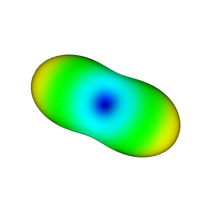
Anisotropic diffusion with discrete 3D EPG — Simulation of signal attenuation due to anisotropic diffusion with discrete 3D EPG#