Isochromat Simulation

The isochromat simulation in Sycomore is based on Hargreaves’s 2001 paper Characterization and Reduction of the Transient Response in Steady-State MR Imaging where limiting cases of the full spin behavior (instantaneous RF pulse, “pure” relaxation, “pure” precession, etc.) are expressed as matrices. The matrices representing building blocks of a sequence are multiplied amongst them, forming a single matrix operator for a repetition. Iterating this process yields a fast simulation of the evolution of a single isochromat and the eigenanalysis of the resulting matrix yields important insights on the steady-state of the sequence.

The matrix operators are represented by the Operator class (C++, Python). Although they can be hand-written, they are designed to be created and combined by the Model class (C++, Python), which also handles the \(T_1\) and \(T_2\) values, and the equilibrium magnetization. All three can be spatially constant or defined at different positions. With a Model, operators can be created using the following functions

• build_pulse (C++, Python)

• build_time_interval (C++, Python)

• or the individual operators forming build_time_interval: build_relaxation (C++, Python) and build_phase_accumulation (C++, Python)

Two operators can be combined: since Sycomore is using column-vectors, the effect of operator \(\mathcal{O}_1\) followed by operator \(\mathcal{O}_2\) on magnetization vector \(M\) is given by \(\mathcal{O}_1 \cdot \mathcal{O}_2 \cdot M\). In a program, operators can be multiplied in-place (O *= P), out-of-place (P = O1 * O2) or pre-multiplied in-place (O.pre_multiply(P), equivalent to O = P*O).

The following code example shows the simulation of a saturation-recuperation experiment: the system is idle for the first 100 ms, a 60° pulse is applied, and the system then relaxes for 1 s. The time step is 10 ms.

Python

import sycomore
from sycomore.units import *

M0 = [0,0,1]
positions = [[0*mm, 0*mm, 0*mm]]
T1, T2 = 1000*ms, 100*ms
flip_angle = 60*deg
step = 10*ms

model = sycomore.isochromat.Model(T1, T2, M0, positions)

pulse = model.build_pulse(flip_angle)
idle = model.build_time_interval(10*ms)

record = [[0*s, model.magnetization[0]]]
for _ in range(10):
    model.apply(idle)
    record.append([record[-1][0]+step, model.magnetization[0]])

model.apply(pulse)
record.append([record[-1][0], model.magnetization[0]])

for _ in range(100):
    model.apply(idle)
    record.append([record[-1][0]+step, model.magnetization[0]])

import matplotlib.pyplot

C++

#include <sycomore/isochromat/Model.h>
#include <sycomore/units.h>

#include <xtensor/xview.hpp>

#include <xtensor/xio.hpp>

int main()
{
    using namespace sycomore::units;
    
    sycomore::Vector3R M0{0,0,1};
    // 1D model at a single position. This can take a more complex form, e.g. for
    // a 3D model at two positions: {{0*mm, 0*mm, 0*mm}, {1*mm, 1*mm, 1*mm}} 
    sycomore::TensorQ<2>positions{{0*mm}};
    auto T1 = 1000*ms, T2 = 100*ms, flip_angle = 60*deg, step = 10*ms;
    
    sycomore::isochromat::Model model(T1, T2, M0, positions);
    
    auto pulse = model.build_pulse(flip_angle);
    auto idle = model.build_time_interval(10*ms);
    
    std::vector<std::pair<sycomore::Quantity, sycomore::Vector3R>> record{
        {0*s, xt::view(model.magnetization(), 0UL)}};
    
    for(std::size_t i=0; i!=10; ++i)
    {
        model.apply(idle);
        record.emplace_back(
            record.back().first+step, xt::view(model.magnetization(), 0UL));
    }
    
    model.apply(pulse);
    record.emplace_back(
        record.back().first+step, xt::view(model.magnetization(), 0UL));
    
    for(std::size_t i=0; i!=100; ++i)
    {
        model.apply(idle);
        record.emplace_back(
            record.back().first+step, xt::view(model.magnetization(), 0UL));
    }
    
    return 0;
}

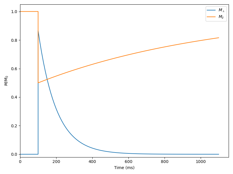
Saturation-recuperation using Bloch simulation