Regular (constant gradient moment) EPG#

In the regular EPG model (C++, Python), the dephasing is reduced to a unitless integer \(k\ge 0\) which represents a multiplicative factor of some arbitrary basic dephasing. The implementation of regular EPG in Sycomore has two high-level operations: apply_pulse (C++, Python) to simulate an RF hard pulse and apply_time_interval (C++, Python) which simulates relaxation, diffusion and dephasing due to gradients. The lower-level EPG operators used by apply_time_interval are also accessible as relaxation (C++, Python), diffusion (C++, Python) and shift (C++, Python). The orders and states of the model are stored in respectively in orders (C++, Python) and states (C++, Python), and the fully-focused magnetization (i.e. \(F_0\)) is stored in echo (C++, Python).

For simulations involving multiple dephasing values (all multiple of a given dephasing), the “unit” dephasing must be declared when creating the model; for simulations involving only a single dephasing value, this declaration is optional, but should be present nevertheless.

The following code sample simulates the evolution of the signal in an RF-spoiled GRE experiment with different phase increments – one model is used per phase increment.

Python

import numpy
import sycomore
from sycomore.units import *

species = sycomore.Species(1000*ms, 1000*ms)

# Sequence parameters
flip_angle=30*deg
TE = 5*ms
TR = 25*ms
phase_steps = [0*deg, 90*deg, 117*deg, 180*deg]
slice_thickness = 1*mm
tau_readout = 1*ms
repetitions = int((5*species.T1/TR))

# Motion to k-space extremity and its associated gradient amplitude
k_max = 0.5 * 2*numpy.pi/slice_thickness
G = k_max / sycomore.gamma / (tau_readout/2)

models = [
    sycomore.epg.Regular(species, unit_dephasing=k_max) for _ in phase_steps]

signals = numpy.zeros((len(models), repetitions), dtype=complex)
for r in range(0, repetitions):
    for index, (phase_step, model) in enumerate(zip(phase_steps, models)):
        phase = (phase_step * 1/2*(r+1)*r)
        
        # RF-pulse and idle until the readout
        model.apply_pulse(flip_angle, phase)
        model.apply_time_interval(TE-tau_readout)
        
        # Readout prephasing and first half of the readout
        model.apply_time_interval(-G, tau_readout/2)
        model.apply_time_interval(+G, tau_readout/2)
        
        # Echo at the center of the readout, cancel the phase imparted by the
        # RF-spoiling
        signals[index, r] = model.echo * numpy.exp(-1j*phase.convert_to(rad))
        
        # Second half of the readout, idle until the end of the TR
        model.apply_time_interval(+G, tau_readout/2)
        model.apply_time_interval(TR-TE-tau_readout/2)

C++

#include <cmath>

#include <sycomore/epg/Regular.h>
#include <sycomore/Species.h>
#include <sycomore/sycomore.h>
#include <sycomore/units.h>

int main()
{
    using namespace sycomore::units;
    
    sycomore::Species species(1000*ms, 100*ms);
    
    // Sequence parameters
    auto flip_angle=30*deg, TE=5*ms, TR=25*ms;
    std::vector<sycomore::Quantity> phase_steps{0*deg, 90*deg, 117*deg, 180*deg};
    auto slice_thickness=1*mm, tau_readout=1*ms;
    std::size_t repetitions = std::lround(5*species.T1()/TR);
    
    // Motion to k-space extremity and its associated gradient amplitude
    auto k_max = 0.5 * 2*M_PI / slice_thickness;
    auto G = k_max / sycomore::gamma / (tau_readout/2);
    
    std::vector<sycomore::epg::Regular> models;
    for(std::size_t i=0; i!=phase_steps.size(); ++i)
    {
        models.push_back(sycomore::epg::Regular(species, {0,0,1}, 100, k_max));
    }
    
    sycomore::TensorC<2> signals({models.size(), repetitions}, 0);
    for(std::size_t r=0; r!=repetitions; ++r)
    {
        for(std::size_t index=0; index!=phase_steps.size(); ++index)
        {
            auto & phase_step = phase_steps[index];
            auto & model = models[index];
            
            auto phase = phase_step * 1/2 * (r+1) * r;
            
            // RF-pulse and idle until the readout
            model.apply_pulse(flip_angle, phase);
            model.apply_time_interval(TE-tau_readout);
            
            // Readout prephasing and first half of the readout
            model.apply_time_interval(-G, tau_readout/2);
            model.apply_time_interval(+G, tau_readout/2);
            
            // Echo at the center of the readout, cancel the phase imparted by
            // the RF-spoiling
            signals(index, r) =
                model.echo() * std::exp(sycomore::Complex(0, phase));
            
            // Second half of the readout, idle until the end of the TR
            model.apply_time_interval(+G, tau_readout/2);
            model.apply_time_interval(TR-TE-tau_readout/2);
        }
    }
    
    return 0;
}

Once the echo signal has been gathered for all repetitions, its magnitude and phase can be plotted using respectively numpy.abs and numpy.angle.

import matplotlib.pyplot

figure, plots = matplotlib.pyplot.subplots(
    2, 1, sharex=True, tight_layout=True, figsize=(8, 8))
for index, (s, phi) in enumerate(zip(signals, phase_steps)):
    plots[0].plot(
        range(repetitions), numpy.abs(s), f"C{index}",
        label=rf"$\phi_{{inc}} = {phi.convert_to(deg):.0f}°$")
    plots[1].plot(range(repetitions), numpy.angle(s), f"C{index}")

plots[0].set(ylim=0, ylabel="Magnitude (a.u.)")
plots[1].set(
    xlim=(0, repetitions-1), ylim=(-numpy.pi, +numpy.pi),
    xlabel="Repetition", ylabel="Phase (rad)")
plots[0].legend()

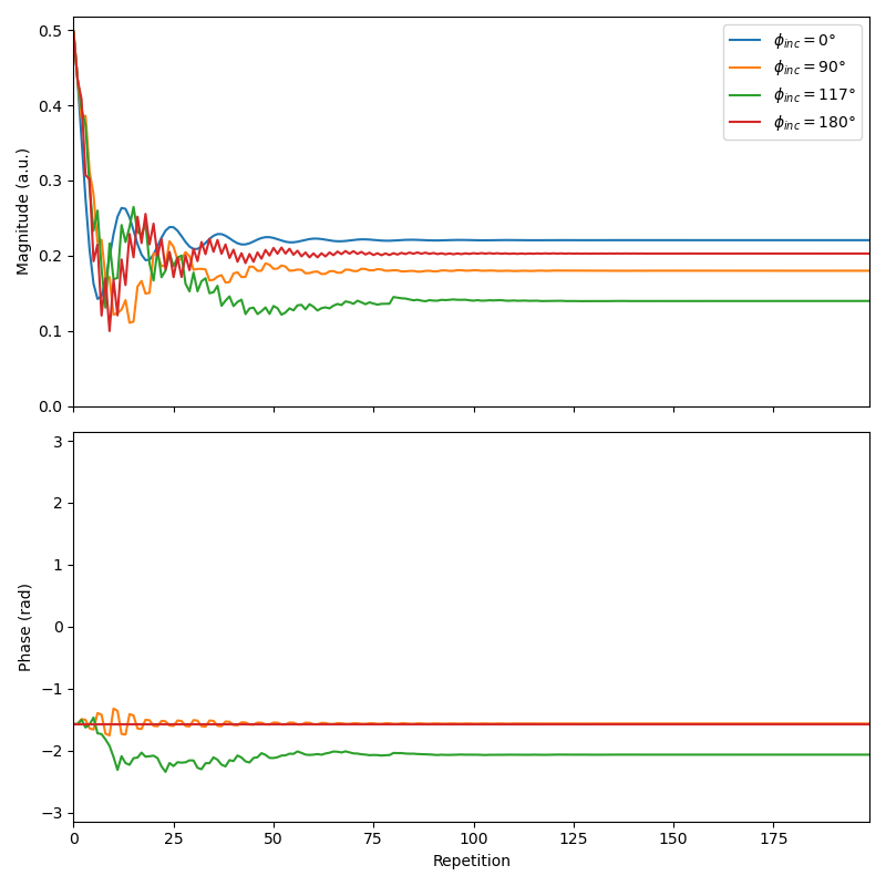
RF spoiling, simulated with regular EPG — Simulation of RF spoiling with regular EPG, using different phase steps#